

Published: Jul 10, 2023 by Boammani Aser Lompo
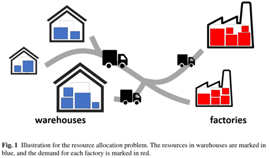
Optimal Transport addresses the problem of moving a mass distribution from one measured space \((X, \alpha)\) to another \((Y, \beta)\).
For instance, consider a city with many bakeries spread across its area. This defines a supply distribution of bread on the city surface \((X, \alpha)\). On the other side, there are numerous bakery stores scattered around the city, defining a demand distribution \((Y, \beta)\). The goal is to determine how to allocate each bakery’s production to the stores in a way that transfers the bread supply to match the bread demand, while minimizing the transportation cost associated with each bakery–store pair \((x,y)\).
More formally, the Optimal Transport objective can be expressed as:
\[\min \int_{X \times Y} c(x,y) \, \mathrm{d}P(x,y) \quad \text{s.t.} \quad P_{\#}^X \gamma = \alpha, \; P_{\#}^Y \gamma = \beta\]where \(P\) is the unknown joint distribution over \(X \times Y\).
In many classical settings, the source distribution \(\alpha\) on \(X\) and the target distribution \(\beta\) on \(Y\) have the same total mass, and the problem can be solved directly.
Here, however, we focus on a more interesting case: unbalanced distributions. Specifically, we will study color transfer between two images that exhibit different color distributions.
In this case, the constraint \(P_{\#}^Y \gamma = \beta\) cannot be strictly satisfied.
First, let’s import the necessary packages.
pip install imageio[pyav]
import numpy as np
import matplotlib.pyplot as plt
from math import floor
import imageio
import warnings
warnings.filterwarnings("ignore")
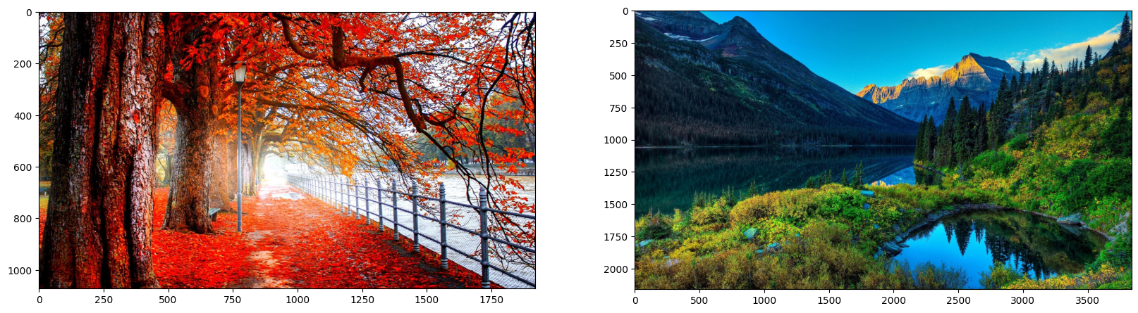
In the variables im1 and im2, we will load images A and B, which we will be working on. They must be in the same directory as this file.
im1 = imageio.imread("example31.PNG")#"img1.jpg")# ,N)
im2 = imageio.imread("example32.PNG")#"img2.jpg")# ,N)

plt.figure(figsize=(20,10))
plt.subplot(1, 2, 1)
plt.imshow(im1)
plt.subplot(1, 2, 2)
plt.imshow(im2)

#convolution through a 3D gaussian Kernel
def K3d(a, kernel):
    res = np.zeros([64, 64, 64])
    for i in range(64):
        KAiK = np.dot(kernel, np.dot(a[i, :, :], kernel))
        for p in range(64):
            res[p] += kernel[i, p] * KAiK
    return res
Now, let’s compute the color distributions of both images and represent them as histograms.
To do this, we discretize the color space \([0, 255]^3\) into a grid of \(64^3\) bins.
hist1 = np.zeros([64, 64, 64])
hist2 = np.zeros([64, 64, 64])

for i in range(im1.shape[0]):
    for j in range(im1.shape[1]):
        [r, g, b] = im1[i, j]
        #replace this line with
        #[r, g, b, _] = im1[i, j]
        #if the image format is in RGBA instead of RGB

        hist1[r//4, g//4, b//4] += 1
for i in range(im2.shape[0]):
    for j in range(im2.shape[1]):
        [r, g, b] = im2[i, j]
        #replace this line with
        #[r, g, b, _] = im1[i, j]
        #if the image format is in RGBA instead of RGB

        hist2[r//4, g//4, b//4] += 1
dx = np.ones([64, 64, 64])
dy = np.ones([64, 64, 64])

lambd = .8;
We now apply the Optimal Transport algorithm, adapted for unbalanced distributions, following Chizat et al., 2016.
- Do not normalize the histograms to apply unbalanced OT (first four lines).
- Normalize if you want to use a Sinkhorn-like approach (which performs better in the end than the actual Sinkhorn).
p = hist1
q = hist2

epsilon = 2
nbr_epoch = 10
b = np.ones([64, 64, 64])

x = np.linspace(0, 1, 64)
y = np.linspace(0, 1, 64)
xx, yy = np.meshgrid(x, y)
kernel = np.exp(-(xx  - yy)**2/epsilon)

batch = 100

u, v = np.zeros([64, 64, 64]), np.zeros([64, 64, 64])
error = np.zeros([nbr_epoch * batch, 2])
seuil = 10

for i in range(nbr_epoch):
    epsilon /= 2
    factor = lambd / (lambd + epsilon)
    for k in range(batch):
        Kb = np.exp(u/epsilon) * K3d(b * dy * np.exp(v/epsilon), kernel)
        #proxdiv = np.divide(p, Kb, where = Kb > 0)
        proxdiv = np.min([np.exp((lambd - u)/epsilon), np.max([np.exp(-(lambd + u)/epsilon), np.divide(p, Kb,
                                                                        where = Kb > 0)], axis = 0)], axis = 0)
        a = np.exp(factor * np.log(np.maximum(1e-60 * np.ones(64), proxdiv)) - u / (lambd + epsilon))
        if (np.max(np.abs(np.log(a))) > seuil):
            u += epsilon * np.log(a)
            kernel = np.exp(-(xx  - yy)**2/epsilon)
            a = np.ones([64, 64, 64])

        KTa = np.exp(v/epsilon) * K3d(np.exp(u/epsilon) * a * dx, kernel)
        err = sum(np.sum(np.sum((b * KTa - q)**2, axis = 0), axis = 0))
        error[i * batch + k, 1] = err

        #proxdiv = np.divide(q, KTa, where = KTa > 0)
        proxdiv = np.min([np.exp((lambd - v)/epsilon), np.max([np.exp(-(lambd + v)/epsilon), np.divide(q, KTa,
                                                                        where = KTa > 0)], axis = 0)], axis = 0)
        b = np.exp(factor * np.log(np.maximum(1e-60 * np.ones(64), proxdiv)) -v / (lambd + epsilon))
        if (np.max(np.abs(np.log(b))) > seuil):
            v += epsilon * np.log(b)
            kernel = np.exp(-(xx  - yy)**2/epsilon)
            b = np.ones([64, 64, 64])

        Kb = np.exp(u / epsilon) * K3d(b * dy * np.exp(v / epsilon), kernel)
        err = sum(np.sum(np.sum((a * Kb - p)**2, axis = 0), axis = 0))
        error[i * batch + k, 0] = err
Next, we compute the new color distribution obtained after applying the Unbalanced Optimal Transport (OT) algorithm.
vx = np.linspace(0, 1, 64)
vy = np.linspace(0, 1, 64)
vz = np.linspace(0, 1, 64)
[vvy, vvx, vvz] = np.meshgrid(vx, vy, vz)

Rvvx = b * np.exp(v / epsilon) * K3d(vvx * np.exp(u / epsilon) * a, kernel)
Rvvy = b * np.exp(v / epsilon) * K3d(vvy * np.exp(u / epsilon) * a, kernel)
Rvvz = b * np.exp(v / epsilon) * K3d(vvz * np.exp(u / epsilon) * a, kernel)

RTx1_J = b * np.exp(v / epsilon) * K3d(np.exp(u / epsilon) * a, kernel)

Rvvx = np.divide(Rvvx, RTx1_J, where = RTx1_J > 0)
Rvvy = np.divide(Rvvy, RTx1_J, where = RTx1_J > 0)
Rvvz = np.divide(Rvvz, RTx1_J, where = RTx1_J > 0)
Coloring the target image
#Nouvelle image
[l, w, _] = im2.shape
im3 = np.zeros([l, w, 3], dtype = int)
for i in range(l):
    for j in range(w):
        #je prends la couleur à changer et je la transforme en élément de I
        [xr, xg, xb] = im2[i, j]//4
        #calcul de la nouvelle couleur
        xxr, xxg, xxb = Rvvx[xr, xg, xb], Rvvy[xr, xg, xb], Rvvz[xr, xg, xb]
        #print(xxr, xxg, xxb)
        #on convertit en entiers
        xxr, xxg, xxb = min(floor(xxr * 256), 255), min(floor(xxg * 256), 255), min(floor(xxb * 256), 255)
        im3[i, j] = np.array([xxr, xxg, xxb])
Here are the two images as they appeared before the color transfer.
plt.figure(figsize=(20,10))
plt.subplot(1, 2, 1)
plt.imshow(im1)
plt.subplot(1, 2, 2)
plt.imshow(im2)
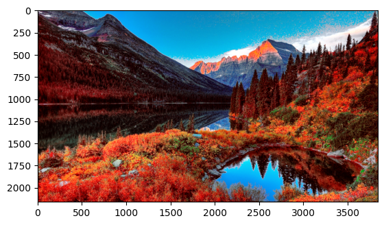
And this is the final result.
plt.imshow(im3)
plt.savefig('example23.PNG')
Share